Introduction
GreenALM is a software package for ab initio modeling of disordered alloys. The package contains an implementation of the density functional theory (DFT) based on a Green’s function framework, also known as Korringa-Kohn-Rostoker (KKR) formalism. KKR-DFT is a general methodology that can, in principle, be applied to any system which can be simulated within DFT. However, the true power of the Green’s function based approach is in its treatment of disordered systems, to which conventional DFT methods cannot be applied directly without extra efforts.
Brief overview of the formalism
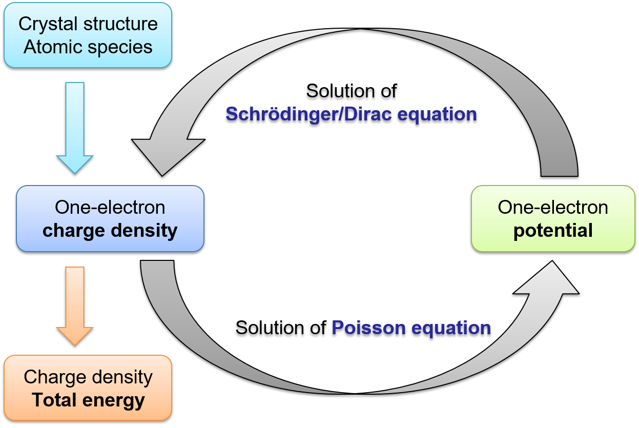
GreenALM implements a usual DFT Kohn-Sham iteration loop, which eventually produces the total energy and the charge density. The only difference from a more widely adopted Hamiltonian approach is that the charge density itself is calculated from the Green’s function instead of a set of wavefunctions. The Green’s function is the primary object of the methodology and can in general be written as follows:
where \(E\) is a (generally complex) energy, \(\Rv_i\) lattice site positions, \(\sigma\) a spin index. Space variables, \(\rv\), are defined with respect to the centers, i.e., \(\rv_i = \rv - \Rv_i\).
In a mathematically rigorous formulation, variables \(\rv_i\), \(\rv_j\) should be restricted to their respective atomic cells, which do not overlap and fill the entire space. However, one can approximate the cells by spheres of the same volume, which amounts to the atomic sphere approximation (ASA). For high-symmetry structures, ASA produces quite good electronic structure and reasonable total energies. The errors introduced by the approximation in case of low-symmetry structures can be systematically reduced by extending the basis set as will be explained below. The current implementation of the method is based on ASA but the approximation is not inherent to the methodology and will be removed in subsequent versions.
Since the code deals with periodic crystal structures, the Green’s function is actually calculated in the reciprocal space,
where the summation is performed over translation vectors, \(\Tv\), vectors \(\qv_i\), \(\qv_j\) are atomic position within the unit cell. Here \(\kv\) belongs to the Brillouin zone (BZ) of the lattice. In practice, only \(\kv\)-points from the irreducible BZ are considered.
The Green’s function is derived from to the scattering path operator (SPO), \(g(E)\), as follows,
where \(L = \{l,m\}\) is a combined orbital index, \(\phi_{iL}(E, \rv_i)\) are partial waves, which are the solutions of the Schrödinger equation inside atomic cells for energy \(E\). The singular part of the Green’s function, \(G^{sing}\), contributes only to on-site terms.
The SPO itself is obtained from the KKR equation inverted in the reciprocal space and integrated over the BZ,
with \(S(E, \kv)\) being the (screened) structure constant matrix (SCM), which is essentially a \(t\)-matrix of the reference system; \(P(E)\) is the potential function related to the single-site \(t\)-matrix as \(P(E) = t^{-1}(E)\). Within ASA the potential function for a spherical potential is diagonal in \(L\). Here we also assumed the periodicity, implying that \(\Rv_i = \Tv + \qv_i\), \(\Rv_j = \Tv' + \qv_j\), with \(\Tv\), \(\Tv'\) being translation vectors.
From the Green’s function the charge desnity is obtained by integrating over energy in the complex plane,
where the integral upper bound, \(E_F\), shows that the contour passes through the Fermi level.
Formally, the lower integration limit here is \(-\infty\). This would, then, include also the core states. In practice, however, it is more conveneint to treat the core state separately (as they are easier to calculate) and to limit the integration to a finite range from \(E_F - D\) to \(E_F\), with \(D\) being the depth of the contour. The integral itself is typically evaluated by a variant of the Gaussian quadratures.
Owing to the symmetry property, \(G(E^{*}) = G(E)^{*}\), the integration is actually performed only over one half of the contour in the upper half-plane and the corresponding factor of 2 is already taken into account in the above equation.
Spectral function
One of the implication of the Green’s-function-only formalism is that, unlike the Hamiltonian-based formalism, it is not possible to directly obtain Bloch states and their energies. To characterize and visualize the electronic structure one can, instead, calculate and plot the Bloch spectral function (BSF) defined as
where the trace implies summation over atomic sites, over \(\{l, m\}\) quantun numbers, and integration over space.
This function, plotted in coordinates \((E, \kv)\) (along a line in \(k\)-space) approximately corresponds to the intensity observed by an angular resolved photoemission spectroscopy (ARPES). The function has peaks at stationary states, with the width of the peaks in \(E\) direction being inversely proportional to the lifetime of these states. For instance, for an ordered system, the peaks of zero width (i.e., \(\delta\)-peaks) will be located right at the positions of the Bloch states, \(E = E_{\nu}(\kv)\).
One particular application of the BSF is visualization of the Fermi surface by plotting \(A(E_F, \kv)\) in a planar cross section of the \(k\)-space.
Integrated over the BZ the BSF gives rise to the density of states (DOS),
which is another useful quantity for analyzing the electronic structure.
Basis set
The basis set currently used in the code are so-called \(2^{nd}\) generation muffin-tin orbitals (MTO). They are smooth site-centered functions consisting of Hankel functions matched with partial waves. Note that another (more advanced) basis set will be used in the subsequent versions of the code.
The size of the basis set depends on two parameters: The maximum value of the \(l\)-quantum number (\(l\)-cutoff), \(l_{max}\), and the number of sites at which the basis functions are defined. The sites usually coincide with real atomic sites but it is possible to add additional centers (“empty spheres”), which is often a necessity for open structures (with a relatively small fraction of volume occupied by atom-centered touching spheres). Examples of common open structures are: simple cubic, diamond and graphite structures, a surface slab with vacuum.
The computational complexity scales is mainly determined by the matrix inversion needed to evaluate the Green’s function matrix in the MTO basis. The linear size of the matrix is \(N = N_{site} N_{lm}\), where the \(N_{site}\) is the total number of sites (including eventual empty spheres) and \(N_{lm} = (l_{max} + 1)^2\) is the total number of basis functions per site. The complexity of matrix inversion is generally \(O(N^3)\). The inversion has to be performed at each \(\kv\)-point of the irreducible BZ and each energy point, which adds a factor of \(N_k N_z\) to the complexity estimate, with \(N_z\) being the number of points on the energy contour.
Total energy
DFT total energy involves three main contributions: one-electron kinetic energy, \(E_{kin}\), electrostatic (Hartree) energy, \(E_{h}\), and the exchange-correlation (XC) energy, \(E_{xc}\). The last term is calculated straightforwardly once the charge density is available and we will not discuss it here in details. The kinetic energy is calculated as the difference between the one-electron and potential energies,
where \(\upsilon_{\sigma}(\rv)\) is the Kohn-Sham potential and the integration is performed over the unit cell. The integral over the unit cell can further be split into integrals over atom cells.
The one-electron energy is obtained directly from the Green’s function,
and the space integration is performed over atom cell \(\Omega_i\).
Integrations over real space are simplified considerably in the ASA because integrals over atom cells turn into integrals over spheres, which are then reduced to radial integrals.
The electrostatic part traditionally poses a challenge because it involves a double integral over space with a non-local kernel with a long range (Coulomb interaction). Within the KKR approach it is split into two parts: intracell and intercell,
The intracell takes into account only electrostatic interactions within an atom cell and can thus be calculated independently for each cell,
where \(\upsilon_{h}(\rv)\) is the Hartree part of the Kohn-Sham potential, \(Z_i\) nucleus charge for site \(i\).
The intercell part can be reduced to the Madelung energy calculated as
where \(Q_{iL}\) are the multipole moments of the charge density within atom cell \(\Omega_i\) and \(M_{iL,jL'}\) is the Madelung matrix. Note that the summation is performed over sites inside the unit cell, whereas periodic images of the unit cell are taken into account by the Madelung matrix.
The Madelung matrix is obtained by Ewald’s summation over all sites of the lattice. The main parameters of the Ewald’s summation are the sizes of the real-space and reciprocal-space clusters and the Guassian parameter \(\lambda\) that controls the relative contributions from the real and reciprocal space clusters.
Note that, strictly speaking, multipole Madelung energy goes beyond the ASA and can be considered as an electrostatic correction. This correction improves the accuracy of the electronic structure considerably, especially for non-cubic or low-symmetry crystal structures. The methodology was referred to as “ASA+M” in some publications.
Coherent Potential Approximation
Disordered systems are currently treated within the coherent potential approximation (CPA). It is a single-site approximation, implying that all alloying effects beyond a single-site (e.g., local atomic environment effects, relaxations, short-range order) are neglected. Nevertheless, this approximation often gives quite good results which can be directly compared to experimental data on single-phase solid solutions. Another advantage is that a CPA calculation is extremely efficient compared to a corresponding supercell setup (which is always an approximation as well). Effectively, the use of CPA increases the overall computational complexity by a constant factor about 5 compared to an ordered system with the same number of species involved.
To perform a CPA calculation one specifies, for a given site, a set of alloy components denoted by index \(\alpha\), with their respective concentrations, \(c_{\alpha}\) (given in atomic fractions). Then, the following set of equations is solved (omitting unnecessary indices),
where in the last two equations we omited indices \(L\), \(i\), and the energy argument for simplicity, having in mind that \(\tilde{g} \equiv \tilde{g}_{iL iL'}(E)\), \(\tilde{P} \equiv \tilde{P}_{\qv_i L L'}(E)\).
Within ASA the average Green’s function on the site is then given by
with \(G_{i,\alpha}(E)\) being the Green’s function of a component \(\alpha\) on site \(i\).
One of the characteristic features of the CPA Green’s function is that its corresponding states visualized by the Bloch spectral function always exhibit finite lifetime. This reflects the fact that electron scattering in a disordered system is inelastic, implying that amplitudes of scattered waves are decaying exponentiall in time and space. At the same time, CPA respects the average translational symmetry and it is, for instance, possible to visualize the Fermi surface of an alloy, which is extremely difficult to do in a supercell representation of the alloy.
From this average Green’s function all other quantities, such as the charge density, the total energy, etc., are obtained. The important point is that both the averaging and CPA equations are carried out on each site independently, which does not affect the complexity scaling with the number of sites. At the same time, the complexity of CPA equations themselves scales linearly with the number of alloy components.
CPA equations are formulated only in term of Green’s functions and related quantities and by itself is independent of the Kohn-Sham equations and DFT in general. A proper solution of both Kohn-Sham and CPA equation requires extra care when it comes to charge self-consistency. One of the issues is that the Madelung energy calculated using the average charges turns out to be incorrect because it misses the electrostatic interaction between individual alloy components. Another of fomulating this is to point out that \(\Av{Q_i Q_j} \neq \Av{Q_i} \Av{Q_j}\), hence the average Madelung energy cannot be simply calculated from the average charges (or multipole moments). To remedy this issue we employ a variant of the screened impurity model (SIM). The model assumes that in a disordered alloy the Madelung potential at a given alloy component \(\mu\) averaged over all sites occupied by this component, \(\Av{V}_{\mu}\), is proportional to the component’s average charge, \(\Av{Q}_{\mu}\). The linear relation can be written in the form of the screened Coulomb potential,
where \(\alpha_{\mu}\) is the screening constant and \(S\) the atomic sphere radius added to the expression to make the screening constant dimensionless. In the CPA all component-related quantities are by construction averaged over realizations of disorder and one can, therefore, simply write \(V_{\mu}\) and \(Q_{\mu}\) for the component’s Madelung potential and charge, respectively.
Since the Madelung energy is calculated not just in terms of charges but in terms of multipole moments, the question is how the latter affect the above relation. It was shown (A. V. Ruban and co-authors) that the linear relation still holds but the slopes are modified and the Madelung energy has to be corrected by an additional factor, screening constant \(\beta_{\mu}\), whose value turns out to be very close to 1 in most of the cases. The final expression for the Madelung energy of a CPA alloy is then given by
The validity of this model has been checked empirically by supercell calculations of various alloy systems. In fact, this is the way the screening constants for alloy components are calculated in practice: One performs a calculation (using the locally self-consistent Green’s function method, LSGF) for a large supercell representing the alloy system and performs a linear regression of the Madelung potential in terms of atomic charge transfers. Given the value of \(\alpha_{\mu}\), screening constant \(\beta_{\mu}\) is determined by precise matching of the CPA and LSGF energies for the same alloy system. Since the concentration dependence of the screening constants is usually smooth (and often quite weak) it is sufficient to do such supercell calculations only for selected compositions (usually the ones that are easy to define by a supercell, e.g., 25%, 50%, 75%, etc.).
Disordered magnetic state
An important particular application of CPA is modeling of magnetic disorder. This is done within the disordered local moment (DLM) model, whereby a pseudo-alloy of spin-up and spin-down components for a given atomic species is formed. The scattering path operator is written as (again, omitting unecessary indices):
with the system of equations being closed by the KKR equation for the coherent potential function.
It is worth noting that an even mixing of the spin-up and spin-down components results in a non-spin-polarized GF but it is very different from the non-magnetic GF for the same system. An important difference is that the lifetime of the states in the DLM state is finite, which would be visible as intrinsic smearing of bands in the plot of the Bloch spectral function.
The DLM approach only works if a given element has a stable local mangetic moment. This is, for instance, the case for bcc Fe or hcp Co. For itinerant magnets, such as fcc Ni, the local mangetic moment is unstable in the paramagnetic state, which means that a DLM calculation would result in a non-magnetic solution.
The DLM model corresponds to the complete disorder of local magnetic moments, which, strictly speaking, corresponds to a high-temperature magnetic state way above the Curie temperature. However, in practice, even right above the Curie temperature only a weak magnetic short-range order is present, and DLM represents a rather good model of the magnetic state even in this case.
For itinerant magnets, such as fcc Ni or fcc Fe at small volumes, the pure DLM approach will result in the non-magnetic solution with zero local mangetic moment. On the other hand, these systems exhibit a strong Curie-Weiss behavior at high temperatures, which is an indication of the local mangetic moments present on atoms. These local moments appear due to thermally induced longitudinal spin fluctuations (LSF). Treating them in general is a hard task requiring resource demanding calculations. However, at high temperatures one can use an approximate description based on the classical picture of the spin moment. This leads to rather simple model of LSF, in which the DFT total energy is extended to the magnetic free energy,
where the magnetic entropy \(S_{mag}\) has a form
with \(M\) being the local magnetic moment and \(\mu\) is the coefficient that depends on the particular behavior of a magnetic species in a given alloy.
Combination of DLM and the above model provides a DLM-LSF description of the high-temperature magnetic state of metallic alloys containing Fe group magnetic elements (Cr, Mn, Fe, Co, Ni).